LLM Training Pipeline for Software: Profiling, Data & Cost

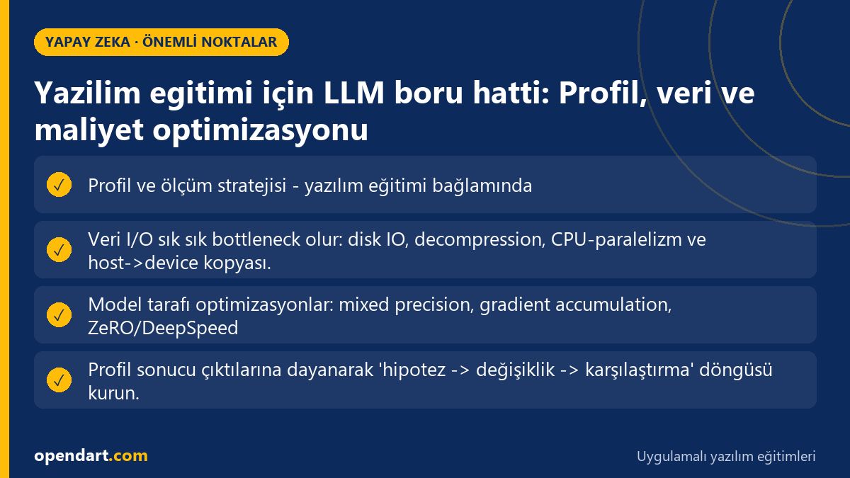
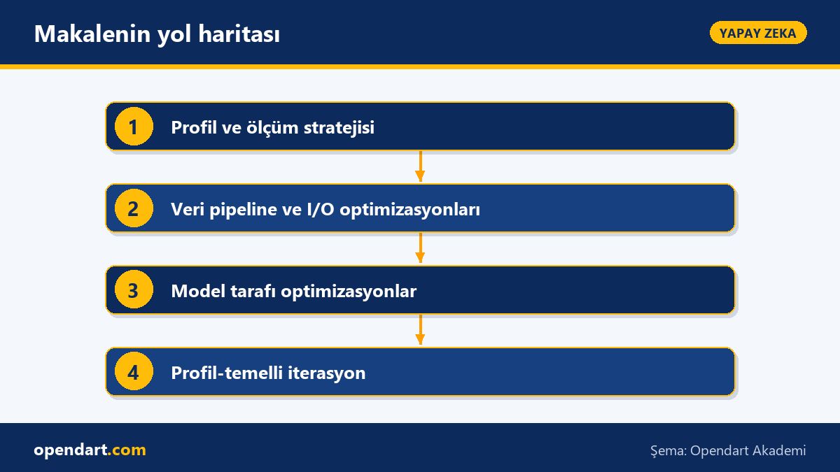
Profiling and measurement strategy — in the software training context

Before you start measuring, clarify target metrics: iterations/sec, p50/p95 step time, peak GPU memory (bytes) and host CPU %user. Measurement tools: NVIDIA Nsight Systems (nsys), py-spy, torch.profiler and nvidia-smi. Concrete step: run a 100-step baseline and compute p50/p95. Example commands: nsys profile --trace=cuda,nvtx -o baseline nsys_report ./train.sh and py-spy top --pid <pid> --nonblocking. Collect and compare these results.

Collecting a code baseline — timing each step and recording GPU peak reveals drift and OOM edge-cases. Add the Python snippet below into your train loop, measure 100 steps and write to CSV:

import time, csv, torch
csvf=open('step_times.csv','w')
writer=csv.writer(csvf)
for i, batch in enumerate(dataloader):
    if i>=100: break
    torch.cuda.reset_peak_memory_stats()
    t0=time.perf_counter()
    loss=model(batch)
    loss.backward()
    optimizer.step(); optimizer.zero_grad()
    torch.cuda.synchronize()
    t1=time.perf_counter()
    peak=torch.cuda.max_memory_allocated()
    writer.writerow([i, t1-t0, peak])
csvf.close()

From this output compute p50/p95 and the memory distribution (numpy.percentile).

Data pipeline and I/O optimizations (webdataset, prefetch, tar shards)

Data I/O often is the bottleneck: disk IO, decompression, CPU parallelism and host->device copy. Tools: webdataset (tar shards), NVIDIA DALI, aiofiles, gpustat and iostat. Why: reading a single large shard increases sequential I/O, while worker parallelism masks decompression time. Measure with iostat -x 1 <device> for disk throughput and latency, and measure dataloader latency in Python with time.time.

Concrete DataLoader config (PyTorch + webdataset) and measurement: num_workers, persistent_workers, prefetch_factor and pin_memory parameters. The example below efficiently loads data from tar shards:

import webdataset as wds
from torch.utils.data import DataLoader
pipe = (wds.Dataset('/data/shards/{000..099}.tar').shuffle(1000)
        .decode('pil').to_tuple('jpg','json'))
dl = DataLoader(pipe, num_workers=8, pin_memory=True, batch_size=32, persistent_workers=True, prefetch_factor=4)
# Ölçüm: her epoch başında iostat ve gpustat ile izleyin
# iostat -x 1 /dev/nvme0n1 &
# gpustat --no-color --watch 1

Change this config (num_workers 2->8, prefetch 2->4) and measure differences in iterations/sec and host CPU usage.

Edge case: pin_memory=True increases host memory usage and can cause OOM on machines with small GPU memory. Mechanism: pinned pages are faster for DMA copies but lock more physical RAM on the host. Experiment by disabling pin_memory and re-running the baseline; check peak host RSS with ps aux --sort=-rss.

Model-side optimizations: mixed precision, gradient accumulation, ZeRO/DeepSpeed

Mechanically, mixed precision (AMP) reduces compute bandwidth and enables tensor cores, lowering time per FLOP and reducing memory requirements. Tools: torch.cuda.amp, Apex (legacy), DeepSpeed and FairScale. Measurement method: compare iterations/sec and peak memory; collect kernel-level timings with a profiler (nsys).

Config example: DeepSpeed ZeRO stage 2 + fp16 and activation checkpointing. Start with this DeepSpeed JSON and run using the deepspeed command:

{
  "train_batch_size": 512,
  "fp16": {"enabled": true},
  "zero_optimization": {"stage": 2, "reduce_scatter": true, "contiguous_gradients": true},
  "activation_checkpointing": {"partition_activations": true}
}
# Çalıştırma: deepspeed --num_gpus=4 train.py --deepspeed_config ds_config.json

Measure with nsys profile --output=ds_trace ./deepspeed_run.sh to get kernel and memcpy details.

Edge case: ZeRO stages can increase CPU-GPU synchronization; with small micro-batches and high gradient_accumulation_steps, communication overhead may dominate. Why: small microbatches generate more optimizer/gradient reduce calls; you should explicitly monitor accumulate step counts, allreduce frequency and overlap parameters. Suggested measurement: compare p95 step time and network I/O (NIC counters or nsys GPU data).

Profile-driven iteration: hypothesis testing, A/B and regression guardrails

Based on profiling outputs, establish a 'hypothesis -> change -> compare' loop. Use experiment tracking like Weights & Biases or MLflow; concrete command: wandb init; wandb.log({'p95_step_time':p95}). Example hypothesis: 'num_workers 8 instead of 4 will improve performance by %X' and test it against a predefined SLO.

Comparison logic: collect 100+ steps per trial, compute p50/p95 and std, then test significance with Mann-Whitney U or bootstrap. Example SQL (for MLflow records or a time-series DB):

SELECT experiment, AVG(step_time) as mean, PERCENTILE_CONT(0.95) WITHIN GROUP (ORDER BY step_time) as p95
FROM runs
WHERE tag='num_workers=8'
GROUP BY experiment;

Monitoring: push step_time to a Prometheus exporter and set a Grafana alert for p95 (alert: p95_step_time > baseline*1.15).

Regression guardrail: add a short 'smoke' profile run in CI before each merge. CI example: run a benchmark job in GitHub Actions, store results as JSON and fail the pipeline if a threshold is exceeded. Example command: python ci_profiler.py --steps 20 --csv out.json ; then check p95 with jq: jq '.p95' out.json | awk '{if($1>0.15) exit 1}'

Frequently Asked Questions

How do I take a quick baseline profile for an LLM fine-tuning software training pipeline?

For a quick baseline: 1) plan a short 100-step run, 2) measure per-step with torch.cuda.reset_peak_memory_stats() + a timer (example code above), 3) run nsys profile --trace=cuda,nvtx -o quick ./train.sh to capture kernel and memcpy analysis, 4) use py-spy top --pid <pid> to find Python CPU hot-spots. These give you p50/p95 and peak memory.

How do I isolate a data I/O bottleneck in a software training pipeline?

To isolate it, use iostat -x 1 /dev/nvme0n1 for disk throughput, gpustat for GPU utilization, and measure dataloader latency inside the train loop (batch start timestamp). If using webdataset or tar shards, vary num_workers and prefetch_factor and compare iterations/sec; try offloading decompression with DALI.

Which metrics should I store in MLflow/W&B for training cost optimization?

Minimum set: iterations/sec, samples/sec (effective batch * iter/sec), p50/p95 step time, peak GPU memory (bytes), host RSS, cost/hour (cloud bill), and GPU utilization. Log these to MLflow or W&B (wandb.log({'p95':p95,'gpu_mem':peak})) and compute cost-per-converge after each experiment.

How do I measure gradient accumulation and mixed precision combination during training?

Method: run three trials with the same seed (baseline, fp16, fp16+accum). For each, record iterations/sec, peak GPU memory and numeric divergence (validation loss difference). Torch AMP example: with torch.cuda.amp.autocast(): loss = model(x); scaler.scale(loss).backward(); scaler.step(optimizer); scaler.update(). Compare nsys traces for these configurations.